Note on Sierpiński Classifier

Elementary note. A Sierpiński space is introduced along with its representability of the open-set functor $O : \mathbf{Top}^{\mathrm{op}} \to \mathbf{Set}$ , then observing how this representability comes out. It is observed that “classifying phenomena” often is encoded within the notion of representability—classifying space is one of such.¹

Table of Contents

Preorders as Thin Categories

Thin categories and preorders

Let $(X, \leq)$ be a preorder. It may be regarded as a thin category by declaring a unique morphism $x \to y$ whenever $x \leq y$ . Reflexivity furnishes identity morphisms; transitivity furnishes composition. Conversely, a small thin category determines a preorder on its object set by

$x \leq y \quad\Longleftrightarrow\quad \mathrm{Hom}(x, y) \neq \varnothing.$

Thus small thin categories are preorders up to isomorphism. Taking the skeleton — identifying objects $x \sim y$ for which $x \leq y$ and $y \leq x$ — produces a poset; hence thin categories are posets up to equivalence. This distinction is minor for many order-theoretic purposes, but it is not vacuous: a preorder may contain distinct yet isomorphic objects when viewed categorically.

Directed subsets as filtered diagrams

A nonempty preorder $D$ is directed if every pair $d_1, d_2 \in D$ admits an upper bound in $D$ : there exists $d_3 \in D$ with $d_1 \leq d_3$ and $d_2 \leq d_3$ .

Viewed as a thin category, this is precisely the condition that $D$ is filtered. A category $I$ is filtered when (1) it is nonempty, (2) any two objects admit a common morphic target, and (3) any two parallel morphisms are equalized by some further morphism. In a thin category the third condition is automatic — there is at most one morphism between any two objects — so a directed preorder is exactly a filtered thin category.

If $D \subseteq X$ is a directed subset of a preorder $X$ , the inclusion $D \hookrightarrow X$ is a filtered diagram in the thin category $X$ . With the convention $x \to y \Leftrightarrow x \leq y$ , the colimit of this diagram, if it exists, is the supremum of $D$ : $\mathrm{colim}(D \hookrightarrow X) = \bigvee D.$

Thus directed joins are filtered colimits in the thin-categorical sense.

Topologies on Preorders via Characteristic Maps

The Alexandrov topology

Let $(X, \leq)$ be a preorder and let $S = \{0 < 1\}$ carry its natural order. The characteristic map $\mathrm{ch}_U : X \to S$ is a morphism of preorders — equivalently, a functor between thin categories — if and only if

$x \leq y,\quad x \in U \quad\Longrightarrow\quad y \in U,$

i.e., if and only if $U$ is upward-closed.

The upper Alexandrov topology on $X$ is therefore

$\tau_{\mathrm{Alex}}(X) = \bigl\{\, U \subseteq X : \mathrm{ch}_U : X \to S \text{ is a morphism of preorders} \,\bigr\},$

whose opens are precisely the upward-closed subsets. In this formulation, upward-closedness is not the primary definition but the order-theoretic expansion of the condition that $\mathrm{ch}_U$ be a functor.

The Scott topology

Let $D \hookrightarrow X$ be a directed subposet — a filtered thin diagram — whose colimit $\bigvee D$ exists in $X$ . The map $\mathrm{ch}_U : X \to S$ preserves this directed colimit if

$\mathrm{ch}_U\!\left(\mathrm{colim}(D \hookrightarrow X)\right) = \mathrm{colim}\!\left(\mathrm{ch}_U \circ (D \hookrightarrow X)\right)$

in $S$ . Since $S = \{0 < 1\}$ is itself a thin category, colimits in $S$ are suprema, so the right-hand side equals $\bigvee_{d \in D} \mathrm{ch}_U(d)$ , and the condition becomes

$\mathrm{ch}_U\!\left(\bigvee D\right) = \bigvee_{d \in D} \mathrm{ch}_U(d).$

Now $\bigvee_{d \in D} \mathrm{ch}_U(d) = 1$ if and only if $D \cap U \neq \varnothing$ , so preservation of this directed colimit is exactly the inaccessibility condition:

$\bigvee D \in U \quad\Longrightarrow\quad D \cap U \neq \varnothing.$

The Scott topology on $X$ is accordingly

$\tau_{\mathrm{Scott}}(X) = \left\{\, U \subseteq X \;\middle|\; \begin{array}{l} \mathrm{ch}_U : X \to S \text{ is a morphism of preorders} \\ \text{that preserves all existing directed colimits} \end{array} \,\right\}.$

Equivalently, $U \in \tau_{\mathrm{Scott}}(X)$ if and only if $U$ is upward-closed and inaccessible by directed joins. The first phrasing is the structural one; the second is its order-theoretic unpacking.

When $X$ is a dcpo every directed subset has a join, so the preservation condition is tested on all directed subsets. When $X$ is not directed-complete, it is tested only on those directed subsets whose joins exist in $X$ .

Comparison: Alexandrov versus Scott

The two topologies are distinguished by which functors $X \to S$ are admitted:

$U \in \tau_{\mathrm{Alex}}(X) \quad\Longleftrightarrow\quad \mathrm{ch}_U : X \to S \text{ is a morphism of preorders,}$

$U \in \tau_{\mathrm{Scott}}(X) \quad\Longleftrightarrow\quad \mathrm{ch}_U : X \to S \text{ is a morphism of preorders that preserves directed colimits.}$

Every Scott-open set is Alexandrov-open, so $\tau_{\mathrm{Scott}}(X) \subseteq \tau_{\mathrm{Alex}}(X),$ and the inclusion may be strict.

Example. Let $X = \mathbb{N} \cup \{\infty\}$ with $0 < 1 < 2 < \cdots < \infty$ , and let $U = \{\infty\}$ . The map $\mathrm{ch}_U$ is monotone, so $U \in \tau_{\mathrm{Alex}}(X)$ . However, the directed subset $D = \mathbb{N}$ has colimit $\bigvee \mathbb{N} = \infty$ , and

$\mathrm{ch}_U(\infty) = 1,\, \bigvee_{n \in \mathbb{N}} \mathrm{ch}_U(n) = 0,$

so $\mathrm{ch}_U$ does not preserve this directed colimit. Hence $U \notin \tau_{\mathrm{Scott}}(X)$ .

This example isolates the distinction: Alexandrov openness detects only monotonicity, while Scott openness further demands compatibility with filtered colimits.

A Worked Example: Five Points

Coincidence of topologies on a finite poset

Let $X = \{a, b, c, d, e\}$ with order generated by $a < b < c, \, a < d,$ and with $e$ incomparable to all other elements.

Since $X$ is finite, every directed subset has a greatest element. Therefore every directed colimit is already attained within the indexing directed subset, and every morphism of preorders $X \to S$ automatically preserves directed colimits. Consequently,

$\tau_{\mathrm{Scott}}(X) = \tau_{\mathrm{Alex}}(X).$

The Scott-open sets are precisely the upward-closed subsets of $X$ :

$\begin{split}\emptyset,\{e\},\{c\},\{c,e\},\{d\},\{d,e\},\{c,d\},\{c,d,e\},\\\{b,c\},\{b,c,e\},\{b,c,d\},\{b,c,d,e\},\{a,b,c,d\},X.\end{split}$

For instance, $\{a, b, c\}$ is not open because $\mathrm{ch}_{\{a,b,c\}}$ is not a morphism of preorders: since $a < d$ yet

$\mathrm{ch}_{\{a,b,c\}}(a) = 1, \, \mathrm{ch}_{\{a,b,c\}}(d) = 0,$

monotonicity would require $1 \leq 0$ in $S = \{0 < 1\}$ , which is false.

The lattice of opens

The topology $\tau_{\mathrm{Scott}}(X)$ , ordered by inclusion, is a complete lattice $(\tau_{\mathrm{Scott}}(X),\, \subseteq).$

Arbitrary joins in this lattice are unions, and finite meets are intersections.

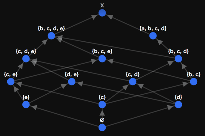The Hasse diagram of this lattice — with fourteen elements — visualizes the topology as an intrinsic ordered object. It is distinct from the Hasse diagram of the original five-element poset $X$ : the latter displays the ordering on elements, while the former displays the ordering on open sets by inclusion. This distinction is often suppressed when one says that finite Alexandrov spaces correspond to preorders; the correspondence is correct, but the topology is itself a nontrivially structured object.

The Sierpiński Space as Classifier

The classifying bijection

Let $S = \{0 < 1\}$ be the Sierpiński Space, two-point set equipped with the Scott, or equivalently, Alexandrov topology $\tau_S = \{\varnothing,\, \{1\},\, S\}$ , where $1$ is the open point and $0$ the closed point. For a topological space $X$ , every subset $U \subseteq X$ has a characteristic function

$\mathrm{ch}_U : X \to S, \, \mathrm{ch}_U(x) = \begin{cases} 1 & x \in U, \\ 0 & x \notin U. \end{cases}$

Since $\mathrm{ch}_U^{-1}(\{1\}) = U$ , the map $\mathrm{ch}_U$ is continuous if and only if $U$ is open. Hence there is a bijection $\mathbf{Top}(X, S) \cong O(X)$ , where $O(X)$ denotes the lattice² of open subsets of $X$ . This bijection sends $f : X \to S$ to $f^{-1}(\{1\})$ , and sends an open subset $U \subseteq X$ to its characteristic function $\mathrm{ch}_U$ .

The bijection is natural in $X$ . If $g : Y \to X$ is continuous and $f : X \to S$ classifies the open subset $U = f^{-1}(\{1\}) \subseteq X$ , then the composite $Y \xrightarrow{\;g\;} X \xrightarrow{\;f\;} S$ classifies $g^{-1}(U)$ , since $(f \circ g)^{-1}(\{1\}) = g^{-1}(f^{-1}(\{1\})) = g^{-1}(U).$

Thus precomposition with $g$ corresponds, under the bijection, to pullback of open subsets along $g$ :

$\begin{array}{ccc}\mathbf{Top}(X, S) & \cong & O(X) \\[4pt]\downarrow{g^\ast} && \downarrow{g^{-1}} \\[4pt]\mathbf{Top}(Y, S) & \cong & O(Y).\end{array}$

Equivalently, the open-set functor $O : \mathbf{Top}^{\mathrm{op}} \to \mathbf{Set}$ is representable with representing object $S$ : $O \cong \mathbf{Top}(-, S)$ ; furthermore, $(S,\{1\})$ is the universal element with respect to $O$ , in a sense that it is the terminal object in the category of elements $\int O:=\Delta \ast\downarrow O$ . ³

Let $\mathbb{T}$ denote a suitable category of spaces for which principal $G$ -bundles are classified by $BG$ , e.g., the category of paracompact Hausdorff spaces, the category of CW complexes, etc. The principal $G$ -bundle functor

${\bf Prin}_G(-):\mathbb{T}^{op}\to {\bf Set}$

sends each topological space $X$ the isomorphism class of principal $G$ -bundle over $X$ .

What bundle theory claims is that there is the representation

$\psi(u): {\bf Ho}\mathbb{T}(-,BG)\cong {\bf Prin}_G;\, [f:X\to BG]\mapsto f^\ast(EG\xrightarrow{u} BG),$

where $u\in {\bf Prin}_G(BG)$ is the universal bundle (indeed, $(BG,u)$ is the universal element).
Or more generally dcpo.
Here we don’t need Yoneda formulation of the category of elements, namely $\int O\cong \mathcal{Y}\downarrow O$ , where $\mathcal{Y}:\mathbf{Top}\to \mathbf{Set}^{\mathbf{Top}^{\mathrm{op}}}$ is the Yoneda functor. We can replace the element-wise definition by Yoneda lemma ${\bf Set}^{{\bf Top}^{op}}({\bf Top}(-,X),O)\cong O(X);\,\alpha\mapsto \alpha_X(id_X)$ .