One found that there is the convention where  denotes the upper-tail critical value such that
  , as a standard notation in probability theory and, especially, in inferential statistics.
This value is often referred to as the upper  -quantile or equivalently, the
  percentile.
While the cumulative distribution function (CDF),  , is fundamental in defining a probability distribution, the use of the right-tail probability for critical values has deep practical and historical roots in hypothesis testing.
Historical Background and Rationale
The primary driver behind this convention is its direct application in hypothesis testing, a framework largely developed by statisticians like Ronald A. Fisher, and Jerzy Neyman and Egon Pearson in the early 20th century. Here’s a breakdown.
Focus on “Significance”
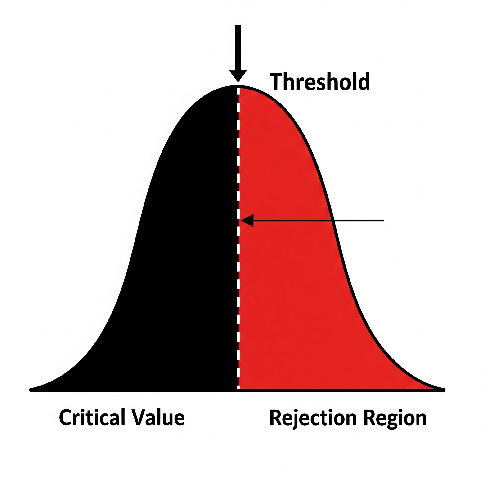
Hypothesis testing is centered around determining if an observed result is “statistically significant.” This often means checking if the result falls into a region of the probability distribution that is considered unlikely or extreme under the null hypothesis ( ). These extreme regions are typically in the “tails” of the distribution, while this does not directly explain why “the right-side” part.
Direct Comparison in Hypothesis Testing
When conducting a hypothesis test, you calculate a test statistic (e.g., a z-score). The decision rule is often to reject the null hypothesis if this statistic falls into the “critical region” or “rejection region.” This region is, in practice, often defined by the critical value . For an upper-tailed test, the rejection region is all values greater than . Therefore, the notation provides a direct and intuitive link between the significance level () and the critical value () that defines the boundary of the rejection region, though this does not explain absolute necessity of “the right-sideness” in defining critical value.
The P-value Concept
The p-value can be interpreted as the probability of obtaining a result at least as extreme as the one observed, assuming the null hypothesis is true. For a one-tailed test where large values of the test statistic provide evidence against , “at least as extreme” translates directly to  , where
  is the observed statistic. The value is the pre-specified significance level, which is the threshold for this probability.
Deep in the p-value
Without limiting our scope to the one-tailed test, can we implicate highly plausible rationale of the right-sideness above the p-value concept?
Axiomatically, a p-value  is a test statistic satisfying
  for every sample point , by which the smaller values give evidence that
  is true, or equivalently, evidence of rejecting .
By restricting our target to the one that is called valid p-value, defined by a p-value that satisfies
![\[P_\theta(p(X)\leq \alpha)\leq \alpha;\quad\forall\theta\in\Theta_0,\foall\alpha\in[0,1],\]](https://blog.icefog.work/wp-content/ql-cache/quicklatex.com-80fee9785f50e69cedce83edfd581f46_l3.png "Rendered by QuickLaTeX.com")
we can explicitly construct the canonical p-value (i.e., “the most common way” of defining valid p-value) along with a given test statistic  , where the large values of
  give evidence that is true.
Theorem 8.3.27 (Casella, George, Statistical Inference 2nd edition).
For each sample point
is a valid p-value.
In the above equation, by setting  against each fixed sample point
  and a given level
 ![\alpha\in[0,1]](https://blog.icefog.work/wp-content/ql-cache/quicklatex.com-31f645b0bd8d16a22d04565382486a12_l3.png "Rendered by QuickLaTeX.com") , it is reasonable to explain that the convention of using for the right-tail probability became dominant in applied statistics because it aligns with the logic and application of hypothesis testing and defining critical regions of significance.
, it is reasonable to explain that the convention of using for the right-tail probability became dominant in applied statistics because it aligns with the logic and application of hypothesis testing and defining critical regions of significance.